Evaluation_Formulae4

3.4.1.1 Evaluation Formulae

For ideal gases with refractive indices differing very little from 1 Gladston-Dale relation (Pavelek, Štětina, 1997) is valid:

,(3.65)

where n – refractive index,

r – density,

K – Gladston-Dale constant.

The Gladston-Dale constant depends on the kind of gas and on the wavelength of the used light. The formula (3.65), as a matter of fact, is the state equation for ideal gas as it mutually joins two state parameters, namely, the refractive index and gas density. The refractive index of dry air with light wavelength of λ = 632,8 nm (for He-Ne laser) is possible to calculate by the formula (Pavelek, Ramík, Liška, 1977 Rottenkolber, 1965):

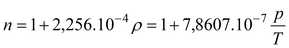,(3.66)

where n – refractive index,

r – density,

p – atmospheric pressure,

T – atmospheric temperature.

The air humidity usually has only a very small influence on the refractive index. For derivation of the air refractive index with respect to its temperature, that is often present in computing formulae for analysis of visualisation records is valid as follows:

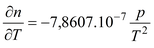,(3.67)

where n – refractive index,

p – atmospheric pressure,

T – atmospheric temperature.

To derive the formulae necessary for quantitative analysis of interferograms we need to describe mathematically the interference origin.

A planar coherent light wave is deformed when passing through transparent surrounding of length l whereas the ideal interferometry considers the wavefront deformation, but ignores the curvature of light beams that should always be perpendicular to the front of the plane light wave. The analysis of the interferograms is based on the equation for optical path difference Δo that was caused by the change of the environment refractive index under the action of optical inhomogenity:

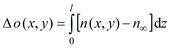,(3.68)

where Do – difference of the optical paths,

l – model length,

n(x, y) – refractive index in x, y point of the phase object,

n_¥ – refractive index in the reference area,

(refractive index of the measuring surrounding without the phase object).

For the two-dimensional transparent object after integration of the equation (3.68) the formula is valid as follows:

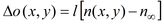.(3.69)

If the deformed light wave of the object beam interferes with the planar wave of the reference beam, an interference patern will occur. For the change of interference order ΔS(x, y) is then valid:

,(3.70)

where ΔS(x, y) – change of the interference order,

l – light wavelength.

The change of interference order ΔS(x, y) gets the values:

ΔS(x, y) = …; –2; –1; 0; 1; 2; … in the positions of bright fringes

ΔS(x, y) = …; –1,5; –0,5; 0,5; 1,5; 2,5; … in the positions of dark fringes.

The presented way of the interference order assignment is valid for the interferometer adjustment to the infinite fringe width in the reference area (in the homogeneous part of the object the change of interference order is ΔS(x, y) = 0) where the reference and object waves in the homogeneous part of the object (see Fig. 3–54) are parallel.

From the equations (3.68) and (3.69) it is possible to derive the ideal interferometry equation from which refractive index n(x, y) in the analysed place is determined as the function of refractive index in the reference area n_∞, change of interference order ΔS(x, y), light wavelength λ and model length l in beam propagation direction.

The ideal interferometry equation is derived on the assumption that the displayed optical inhomogenity causes a negligibly small deviation and displacement of the light beam, and has the form:

,(3.71)

where n(x, y) – refractive index in x, y point of the phase object,

n_¥ – refractive index in the reference area,

DS(x, y) – change of interference order,

l – light wavelength,

l – model length.

To analyse the interferograms we must know the physical relation between the state parameters (density, temperature, concentration) and distribution of the refractive index in the optical inhomogenity caused by the change of these parameters.

From the distribution of refractive index n(x, y) we can determine temperature distribution under constant pressure by state equation (Pavelek, Ramík, Liška, 1977):

,(3.72)

where T(x, y) – temperature distribution,

T_¥ – atmospheric temperature in the reference area,

p_¥ – pressure in the given space,

s – interference order,

l – light wavelength,

l – model length.